Machine Learning (ML) is typically seen as a “black-box” approach to an otherwise intractable problem that you can't analytically model nor obtain mathematical insights. In our recent paper, we show that instead of this black-box alternative pathway to high-performance solutions and bypass good-old hardcore mathematical analysis, ML can actually be a complementary tool to guide human analytical thinking and advance Optics and other disciplines that are deeply rooted in solid foundations in Physics and Mathematics.
In particular, we (led by our Ph.D student Remi Qirui Fan) show that by making sense of the optimized neural network model configurations and combine with domain-specific knowledge, one can obtain new and deeper analytical insights into nonlinear distortions in optical signals and how we can design digital signal processing(DSP) algorithms to increase optical communications speed. The model is experimentally verified in an actual 815-km optical transmission testbed. The new algorithm beats the state-of-the-art(SOTA) and is the first demonstration of a practically implementable algorithm that improve transmission capacities. This work is an example of interpretable ML in Physical Science and Engineering.
Interpretable ML and applications in Physical Sciences and Engineering
With the surge of ML research and applications and how they are fundamentally transforming every aspect of our society, algorithms outperforming humans is no longer enough. We also need to understand why that trained neural network of yours is able to arrive at that classification it makes. Why do we care? That's because if you want ML to be really applied to more important tasks such as medicine, finance, law (as supposed to neural nets that distinguish between cat and dog pics), there are legal, ethical and regulatory requirements that one is able to explain what the algorithm is doing and how it arrives at the conclusion. This is a recent sub-branch of ML research called interpretable ML and is receiving more attention as people try to adopt ML in more important and mission-critical tasks. In other words, we don't want ML to be the "black box" algorithm that out-beat humans but we don't have the slightest clue on what they are actually doing. A great review article on interpretable ML can be found here.
A really fascinating emerging area under interpretable ML is ML-/data-driven Science and Engineering discovery. Schmidt and Lipson demonstrated for various physical systems ranging from simple harmonic oscillators to double-pendula, one can capture motion-tracking data, take empirical time-derivatives, use evolutionary algorithms to build equations that gives accurate prediction results. Without any prior knowledge about physics, kinematics, or geometry, the algorithm discovered Hamiltonians, Lagrangians, and other laws of geometric and momentum conservation applications in Physical Sciences. Champion et al took a further step and demonstrate how one can learn the right frame of reference to transform high-dimensional to low-dimensional time-series data and then discover equations governing the dynamics of Lorenz, reaction diffusion and pendulum model.
Iten et al also use neural networks SciNet to find the physically relevant parameters, exploits conservation laws to make predictions, and can help to gain conceptual insights. In one instance, SciNet provides accurate predictions of the angular momentum of two balls after they have collided. That’s only possible using the conservation of momentum, a version of which SciNet appears to have discovered. In another example, one feeds SciNet with the time series data of the angles of Mars and Sun as seen from Earth into a neural network. Upon convergence, the network actually stores the angles of the Earth and Mars as seen from the Sun in the two latent neurons. This suggests that SciNet had learnt that taking the Sun as the static frame of reference is more appropriate i.e. the machine (re)discovers Copernicus' conclusion that the solar system is heliocentric i.e. Sun at the center.
A main take away among all these works is that "In the end, we still need a scientist to look at this and say, this is interesting," said Lipson. For example, you'd still need someone with a background in astronomy and math to look at the stored angles and realize what has the machine really learnt. In other words, humans are still important in the process of knowledge discovery and can't be completely taken away.
"In the end, we still need a scientist to look at this and say, this is interesting," said Lipson. In other words, humans are still important in the process of knowledge discovery and can't be completely taken away.
Before we go into the details of how interpretable ML help advance optical communications, let's briefly discuss the background to provide some context.
Fundamental bottleneck in Optical Communications
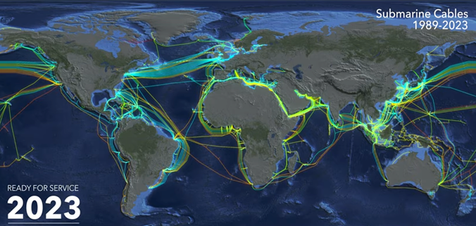
More people are enjoying fiber-to-the-home now and holding a piece of optical fiber for the first time. But that's not even close to the complete picture: All forms of communications, at the end, go through optical links: from google search to AR/VR applications. Data centers are all linked by optics now. A lot of homes have fiber-to-the-homes installed and so some of you actually see an optical fiber for the first time in your life. Optical links are being laid worldwide at unprecedented rates
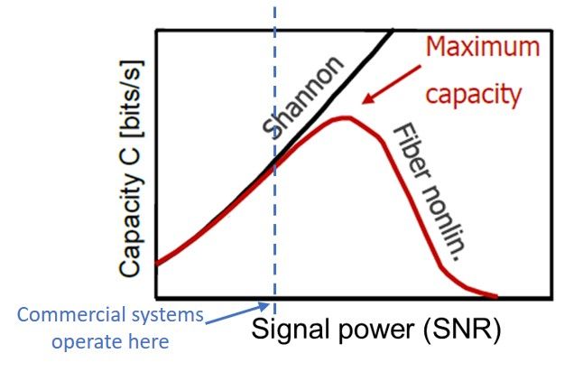
You might have heard that the capacity $C$ of a link is
$$ C=log_2(1+SNR)$$
where SNR is the signal-to-noise ratio. This is the classic Shannon capacity limit. Therefore, as signal power increases, we will get faster connections. However, its not so simple in reality. Optical transmission capacity will peak at some power level and go back down because of increasing fiber nonlinear distortions. Fiber nonlinearity is the biggest hurdle and is perhaps the most fundamental bottleneck of optical communications since its invention 50 years ago.
Fiber nonlinearity is perhaps the most fundamental bottleneck of optical communications since its invention 50 years ago.
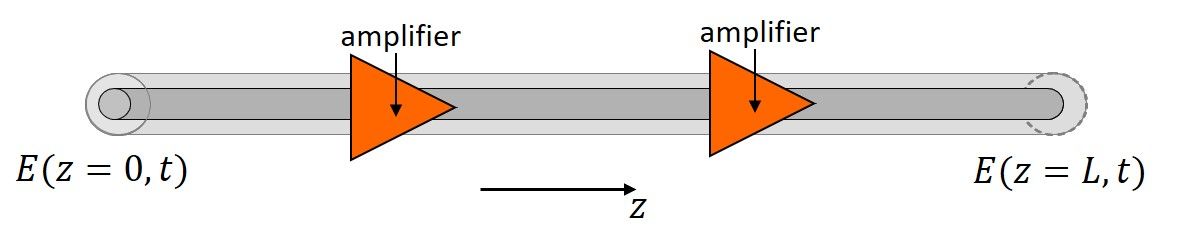
So, what is fiber nonlinearity? In optical communications, we typically denote a signal (or a time waveform) in a fiber at distance $z$ from the transmitting end as $E(z,t)$. The signal is electromagnetic(EM) fields by nature and are complex-valued quantities. (Complex-valued signals is just a notational convention. A complex signal $a(t)+jb(t)$ merely means the actual signal is $a(t)cos(2\pi f_c t)-b(t)sin(2\pi f_c t)$ where $f_c$ is the carrier frequency of the signal. For optical communications, $f_c$~ 193 THz. For Wifi, $f_c$~ 2.4 or 5GHz and FM radio operates at $f_c$~ 88 to 110 MHz just to give a few examples.)
The evolution of $E(z,t)$ along the fiber (or along $z$) follows the famous Nonlinear Schrodinger Equation(NLSE)
$$\frac{\partial E(z,t) }{ \partial z} = -\frac{\alpha}{2}E(z,t)-j\frac{\beta_2}{2}\frac{\partial^2 E(z,t)}{ \partial t^2} +j\gamma |E(z,t)|^2 E(z,t)$$
The term with $\alpha$ denotes signal loss along propagation. This is largely addressed with decades of advances in fiber manufacturing (signal loss in fiber have pretty much reached the theoretical limit) and optical amplifiers. The term with $\beta_2$ denotes chromatic dispersion(CD) where pulses disperse and overlap with each other along propagation. This is a linear effect that can be characterized by a transfer function $ H(\omega)=e^{j\omega^2 \beta_2L/2} $ where $L$ is the total propagation length. At the receiver, one can largely undo the effects of $ H(\omega)$ by multiplying $H^{-1}(\omega)$ to the received signal spectrum to cancel out each other. For the sake of completeness, signal loss is also a linear effect.
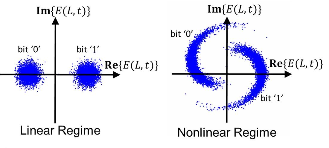
The last term with $\gamma$ is a lot more interesting. As it turn out, since the EM fields are concentrated in the core of optical fibers, the interactions between the EM fields and the fiber molecules can be so strong that the refractive index of the fiber start to increase with signal power! This phenomenon is called Kerr nonlinearity and $\gamma$ is the fiber nonlinearity coefficient that measures the strength of this phenomenon. The refractive index change translates into additional phase noise in the signal and such distortions actually scales up with signal power. This in turn creates a situation where the SNR degrades as signal power goes up. Consequently, transmission capacity does not go up like $ C=log_2(1+SNR)$, but it will peak at some power level and go back down because of increasing nonlinear distortions.
Fiber nonlinearity induces additional phase noise to the signal and such additional distortions actually scales up with signal power. This in turn creates a situation where the SNR degrades as signal power goes up.
State-of-the-art approach and its limitations
First of all, the sole objective of all signal processing in Telecomm. is to recover the transmitted signal from the received signal i.e. to estimate $E(0,t)$ from $E(L,t)$.
Well, how do we do that? To answer this question, let's first understand how we can calculate the received signal $E(L,t)$ from the transmitted signal $E(0,t)$. One can numerically solve the NLSE by iterating the linear operation D (that includes loss and CD) and the nonlinear operation N (that includes fiber nonlinearity) on $E(0,t)$ as shown in the figure below. In each iteration, the algorithm sequentially calculates the linear and nonlinear effects on the signal over distance $\Delta z$, which is called the step size.
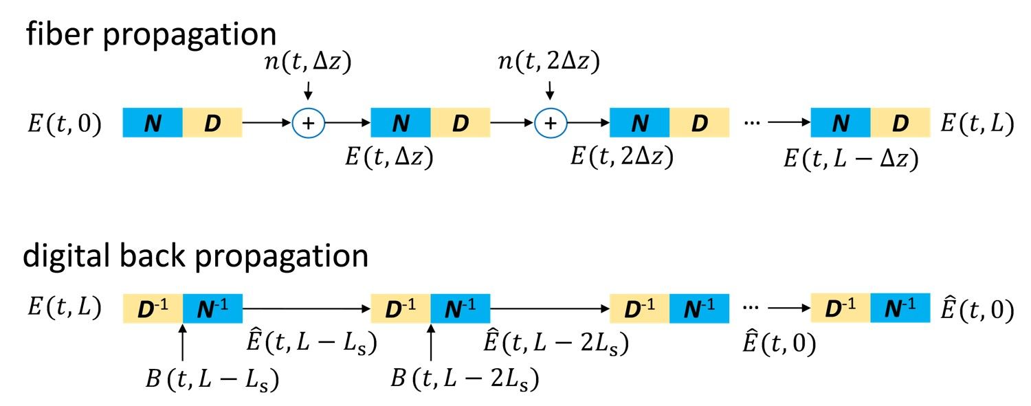
Therefore, to un-do all the linear and nonlinear effects and recover $E(0,t)$ from $E(L,t)$, the state-of-the-art approach is called digital back-propagation(DBP) (Sorry this is not to be confused with back-propagation in the ML community in which gradients are propagated back from the output layer to input layer to update weights and biases). DBP is an algorithm that essentially reverses the linear and nonlinear operations of the NLSE iteratively (basically un-doing whatever the fiber does to the signal), hence its name. It is an inconvenient coincidence that different communities use similar terminologies to describe very different things.
DBP dates back to 2008 when it was first proposed by my research group when I was a Ph.D. student and other groups. Typically, the step size $\Delta z$ is chosen as the length of 1 span of fiber (around 80 km) in research papers and this benchmark is called 1 step-per-span(1-StPS) DBP.

Despite DBP being out there in the research community for a decade already, there's still no commercial Telecomm. line cards using DBP. This is because
- Additional noise from amplifiers along the link complicates the whole propagation dynamics and effectiveness of DBP. The signal propagation dynamics is actually $$\frac{\partial E(z,t) }{ \partial z} = -\frac{\alpha}{2}E(z,t)-j\frac{\beta_2}{2}\frac{\partial^2 E(z,t)}{ \partial t^2} +j\gamma |E(z,t)|^2 E(z,t)+n(z,t)$$ where $n(z,t)$ are additive white Gaussian noise process. This whole thing become stochastic and you can't perfectly undo the fiber effects since you get a noisy+distorted signal to work with.
- We are talking about > 400 Gb/s transmission for modern optical links. The processing speed makes DBP computationally very complex thus highly unfavourable to be implemented in practice. In fact, optical communications is the field that push the speed limits of computer chips – nobody else needs signal processing at that kind of speed.
- The gain is too small, especially in practical wavelength division multiplexed (WDM) systems carrying multiple optical signals with different wavelengths (or different carrier frequencies $f_c$). Also, because of point 2 above, one is restricted to single channel signal processing and there's no place for joint channel processing in practice.
Machine Learning-enabled DBP optimization
Since the DBP algorithm are interleaving linear and nonlinear operations, its naturally in a form of a deep neural network (DNN) as shown in the figure below ( Well, not exactly a typical DNN since the nonlinear operation here $\sigma$ is phase rotation as supposed to typical sigmod, ReLU activation functions). Nevertheless, when viewed this way, one can't help to wonder: what if we see the DBP as a DNN and try to learn all the parameters of the DBP such as the linear filter taps and the phase rotation for each step? How much can ML improve DBP performance? This idea is originally proposed by Hager and Pfister and we're here to experimentally demonstrate it for the first time and provide deeper analytical insights.
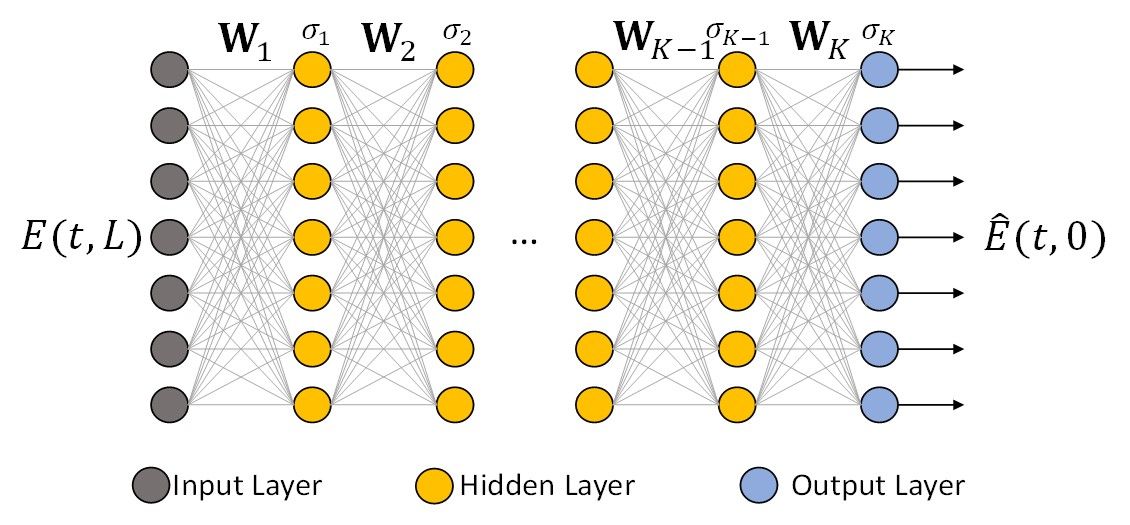
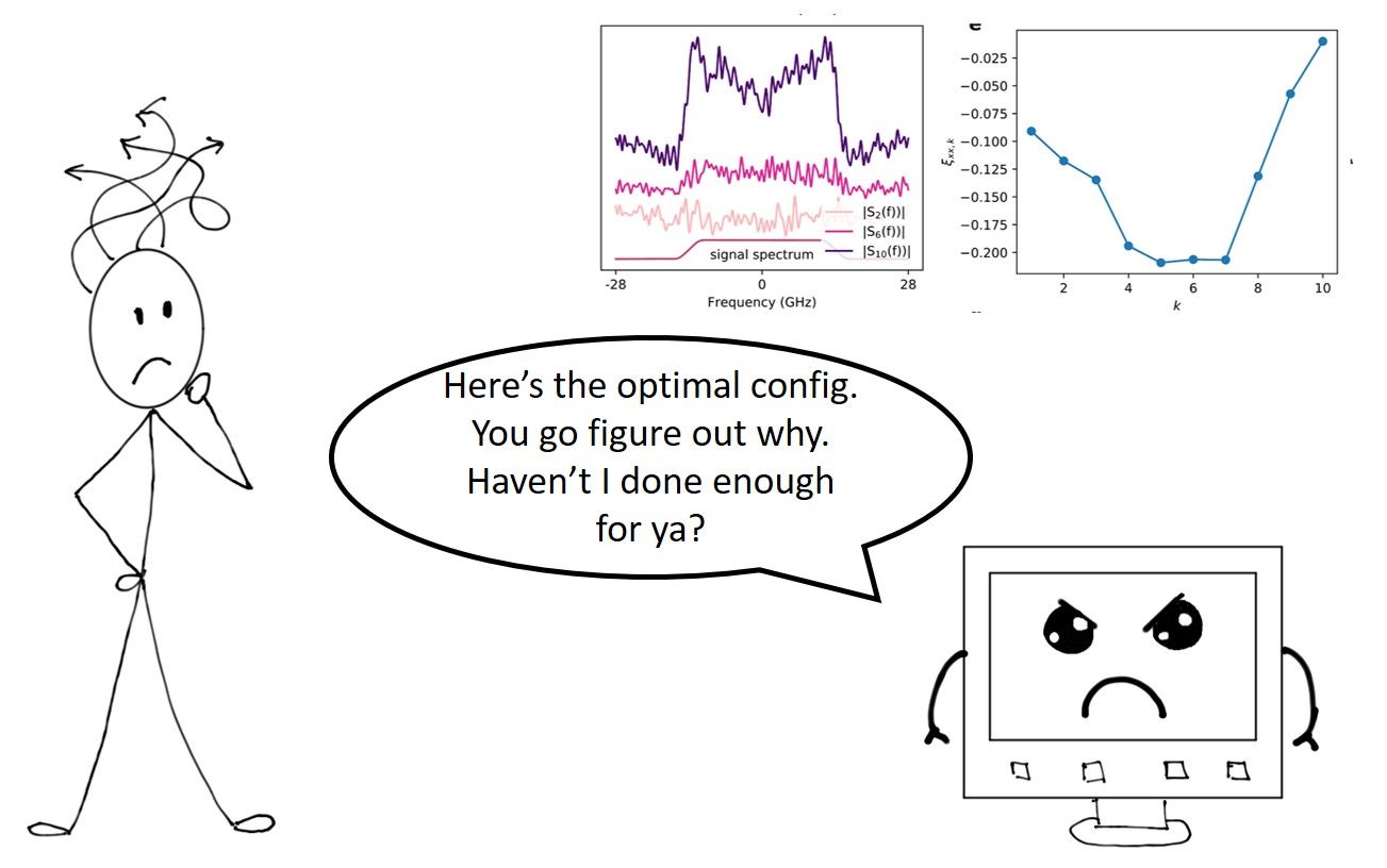
Incorporating domain-specific knowledge: Now, because we know from NLSE and DBP that the $k^{th}$ linear step correspond to a linear filtering with spectrum $S_k(f)$, the weights and bias $W_k$ of the DNN should resemble a linear filter. We therefore restricted $W_k$ to be a Toeplitz matrix so that multiplying by $W_k$ is equivalent to linear filtering by $S_k(f)$. The nonlinear operation at the $k^{th}$ step is chosen to be the phase de-rotation $\sigma_k=exp(-j\gamma\xi_k \Delta z |\cdot|^2)$. In this case, the spectra shapes $S_k(f)$ and $\xi_k$ are to be learnt by Machine Learning.
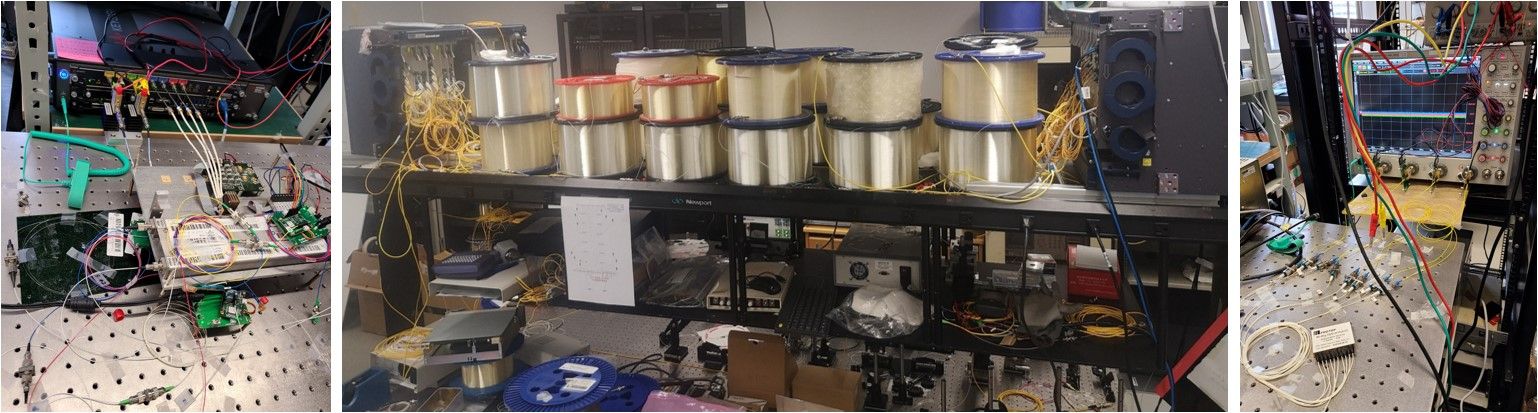
We transmit 28Gbaud 16-QAM signals (i.e. 224 Gb/s per channel over two signal polarization) over 815 km of fiber. We chop the received signals into blocks of vectors as input. The input to the DNN-based DBP is the sampled received signal with sampling rate of 2 samples/symbol. We use the 32768 symbols for training and 25 copies of the another 32768 symbol sequence for testing. To take into account the dispersive and pulse overlapping nature of the received signals, neighboring mini-batches are formed with overlapping vectors and 60 neighboring samples are appended to the two ends of each input. We tuned the input vector size and linear filter length and show that 128 samples per input and 121 taps are optimal settings across most experimental setups studied in our work. We chose the AdaBound optimizer so as to separately tune its initial- and final learning rates. The number of layers in the deep neural network is equivalent to the number of DBP steps. We choose MSE (between the network output and the original symbol sequence) as the cost function. The DNN-based DBP is optimized by using 200 epochs with step size 0.01.

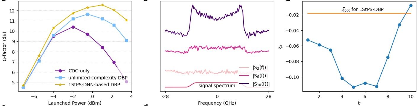
Results for single channel transmissions over a link of 815 km are shown in the left of the figure below. We typically quantify transmission performance using Q-factor, which is related to the bit error ratio(BER) by $Q=20\log_{10}(\sqrt{2}erfc^-1 (2BER))$ where erfc is the complementary error function, and in turn closely relates to transmission capacity. It can be seen that 1-StPS DNN-based DBP already outperform unlimited-complexity DBP (meaning choosing step size $\Delta z \rightarrow 0$) by 0.9 dB. The gain is over 2 dB if one compares with a CD compensation (CDC)-only algorithm. In long-distance optical communication systems, improving the Q-factor by 0.2 dB translate into significant performance improvements and cost savings from an operator point of view.
The converged linear filter spectra $S_k(f)$ and phase de-rotation coefficients $\xi_k$ are also shown in the middle and right of the figure below. Note that the converged amplitude responses have a ‘M’-shaped feature and become more apparent at later stages of the DNN-based DBP. Furthermore, the optimal $\xi_k$ learnt by machine learning are have a ‘U’-shaped structure so that the nonlinear phase de-rotation is larger in the middle stages.
The approach also works for wavelength-division-multiplexed (WDM) transmissions which are standard in commercial systems and the results are shown below for a 5-channel system over the same experimental setup. The performance gain of DNN-based DBP is 0.25 dB over unlimited-complexity DBP and a total gain of 0.85 dB over CD compensation(CDC)-only. The ‘M’-shaped and ‘U’-shaped feature are also clear.
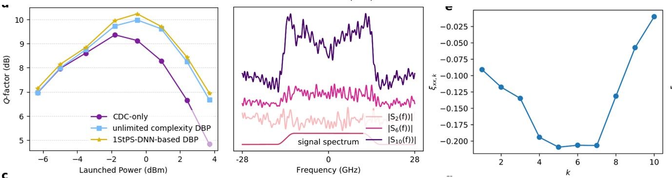
The WDM results outperform SOTA and are the first demonstration of a single-channel signal processing algorithm that actually produces sizable gains in practical WDM environments. They alone are already an important demo of a practically implementable algorithm that can potentially break the long-standing barrier of fiber nonlinearity in optical communication systems.
Interpretable ML and deeper understanding of fiber nonlinearity compensation
The story does not stop here. Looking at the optimal configurations of the filter shape and the phase rotation coefficients, one can't help but notice: why are the filters $S_k(f)$ M-shaped and $\xi_k$ U-shaped?
In most applications, ML are ‘black-box’ models with excellent predictive power but it is difficult to inquire how they work exactly and why they produce such good results. However, in our case, the ‘M’-shape and ‘U’-shape features are clear mathematical structures that strongly suggests certain hidden dynamics of DBP yet to be better understood. The ‘M’-shaped filter indicates that the optimal linear filter exhibits some high-pass feature which become more pronounced at later stages of the DNN-based DBP. An explanation for this phenomenon is that there exists an additional undesired term with a ‘$\cap$ ’-shaped spectrum that grows with the DNN-based DBP stages that the ‘M’-shaped filter tries to compensate. On the other hand, the ‘U’-shaped $\xi_k$ suggests that the nonlinear phase de-rotation is small at the beginning and towards the end of the DBP but is larger in the middle stages. This can imply that the beginning and end stages of DBP are more prone to noise and distortions and hence phase de-rotation based on instantaneous signal power may not be effective. The overall optimized DNN-based DBP configuration from ML seems to suggest that noise and distortion accumulations play a hidden yet pivotal role in the effectiveness of DNN-based DBP.
We proceed to analyze noise and distortion accumulations in DBP to try to explain the optimal DNN-based DBP configurations discovered by machine learning. The detail derivations can be found in the paper where we denote $E_z$ as $E(z,t)$ and $CD^{-z}(\cdot)$ means inverting the effect of CD over a distance $z$. In the limit of large number of steps with $\Delta z \rightarrow 0$ (we called this the distributed amplification limit), the transmitted signal estimate is given by
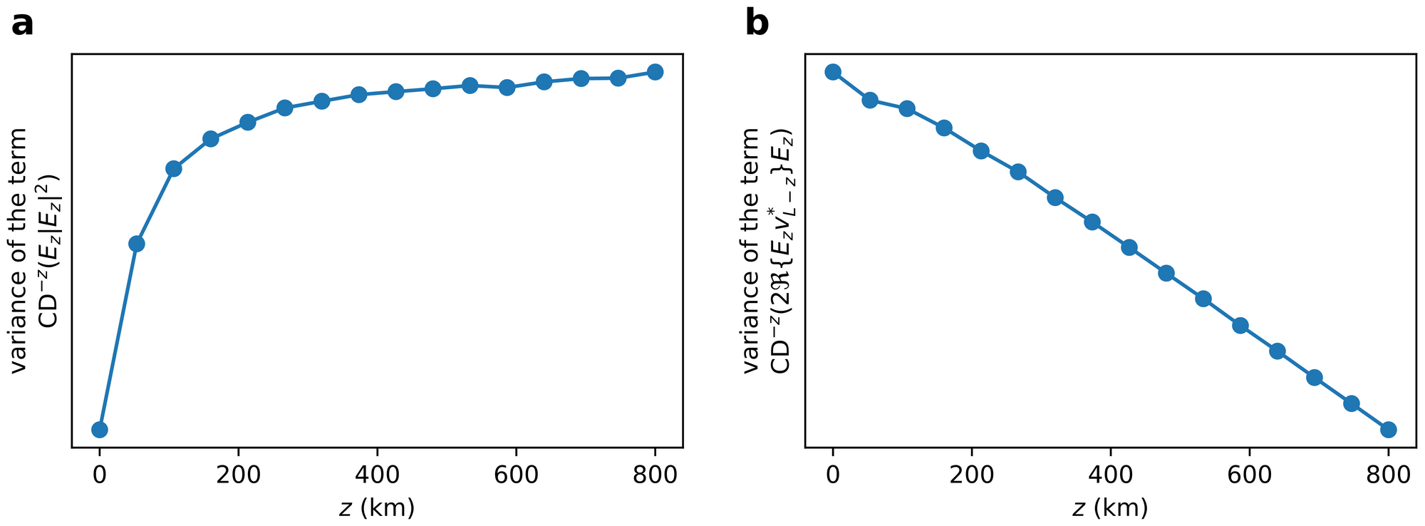
$$\hat{E}_0=E_0+j\gamma\int_0^L (1-\xi_z)CD^{-z}(|E_z|^2 E_z)-2\xi_z CD^{-z}(\Re\{E_zv^*_{L-z}\}E_z)dz + v_L $$
where $v_L$ corresponds to the total ASE noise in the system and the term $j\gamma\int_0^L CD^{-z}(|E_z|^2 E_z)dz$ actually corresponds to the nonlinear phase shift due to the signal and is largely compensated by other algorithms in practical systems. The other terms $j\gamma\int_0^L \xi_z CD^{-z}(|E_z|^2 E_z)dz$ and $j\gamma\int_0^L 2\xi_zCD^{-z}(\Re\{E_zv^*_{L-z}\}E_z)dz$ are the major nonlinear impairments that degrades transmission performance. As the variances of the noises and distortions are typically used to characterize overall system performance, the figure below shows the simulated variances of $CD^{-z}(|E_z|^2 E_z)dz$ and $2CD^{-z}(\Re\{E_zv^*_{L-z}\}E_z)dz$ as a function of $z$ and it can be seen that one of them increases with $z$ while the other decrease with $z$. As $\xi_z$ control the relative strengths of $CD^{-z}(|E_z|^2 E_z)$ and $CD^{-z}(\Re\{E_zv^*_{L-z}\}E_z)$ in the overall nonlinear distortions in $\hat{E}_0$ , we can now appreciate why $|\xi_z|$ is smaller at the beginning and end of the GDBP stages and larger in the middle as shown above i.e. the ‘U’-shaped profile. This feature can be intuitively interpreted by noting that
1) the nonlinear phase de-rotation at each DBP stage is not perfect due to ASE noise and such imperfections accumulate throughout the whole DBP chain. Imperfections at the early DBP stages (corresponding to $\xi_z$ for $z \approx L$ ) accumulates the most in the final signal estimate $\hat{E}_0$ and therefore $\xi_z$ should be small for $z \approx L$ to minimize such accumulation, and
2) towards the end of the DBP, the signal amplitude is already heavily distorted and quite different from the original signal due to noise and accumulation of imperfect compensation from preceding DBP stages. Therefore, the phase de-rotation at the end of the DBP stages (corresponding to $\xi_z$ for $z \approx 0$ ) will not be accurate and hence $\xi_z$ should be small for $z \approx 0$ to prevent the production of additional distortions.
3) In addition, since the imperfect phase de-rotations cannot completely eliminate the nonlinear distortion term $|E_z|^2 E_z$ , they continue to grow within the DBP stages and accumulate at the end of the algorithm. As $|E_z|^2 E_z$ has a ‘$\cap$ ’-shaped spectrum, an inverted-shaped spectrum to partially equalize the distortions will be more beneficial than a pure CD compensation operation. Furthermore, since $|E_z|^2 E_z$ has 3 times the bandwidth of $E_z$ , one should simply filter out the out-of-band distortions at each DBP stage. This two factors together explains why the overall linear filter of GDBP exhibit the ‘M’-shaped features as shown in the optimized configurations above and how the shape is more apparent towards the later stages of the DNN-based DBP.
The new insights: The analysis from the ML-optimized configurations illustrate that the optimal linear filter of DNN-based DBP does not merely equalize CD. It is in fact a tradeoff between compensating CD of the signal and mitigating the 3rd-order nonlinear distortion term $|E_z|^2 E_z$ as it accumulate along the DBP stages. Similarly, the optimal nonlinear phase de-rotation actually attempts to strike a balance between reversing the nonlinear phase during propagation and minimizing additional phase noise accumulations along the DBP stages due to corrupted signal power levels.
In a nutshell, the Machine Learning-inspired analysis reveals that the original design philosophy of DBP as iterative linear/nonlinear compensation of fiber propagation effects does not paint the whole picture. Rather, the optimal signal processing should undo the propagation effects as well as manage the self-inflicted additional distortions accumulated within the interleaving DBP steps.
Conclusions and Take Away
- ML enable the first experimental demo of a practically feasible algorithm that mitigates fiber nonlinear effects and improves multi-channel optical transmission capacity. It outperforms SOTA and is a good step towards pushing the fundamental limit of optical communications.
- the learnt parameter configurations from ML in turn guided us to analyze the interplay between CD, nonlinearity and noise and led to deeper theoretical insights and interpretations of signal processing in nonlinear optical communication systems (the explanation of the M- and U-shapes and their implications). This shows that ML can help advance our analytical understanding of Physical Science and Engineering problems (assuming there's a human with domain-specific knowledge to work alongside) and is not always just an easy way out to arrive at intelligent solutions for intractable systems.
- Throughout the work, we also realize that the ADAM optimizer from Tensorflow 2 has issues for complex-valued input. This is because special care is needed to calculate complex-valued derivatives (called Wirtinger calculus) for gradient descents in any optimizer. We reported this issue at https://github.com/tensorflow/tensorflow/issues/38541 . We will be submitting a new code to fix the ADAM optimizer for complex-valued inputs.
Contact: eeaptlau@polyu.edu.hk ; https://alanptlau.org/